Creating and simulating a DFBA model

This tutorial demonstrates how to build and simulate a DFBA model corresponding to the growth of a single strain of Escherichia coli (based on the iJR904 genome-scale model) under anaerobic conditions with glucose and xylose as limiting carbon substrates.

This example can be adapted to other DFBA models by modifying the choice of genome-scale model, relevant kinetic variables, and exchange fluxes.

from os.path import dirname, join, pardir

from cobra.io import read_sbml_model

from dfba import DfbaModel, ExchangeFlux, KineticVariable

1. Dfba model

Specify path for loading file containing genome-scale metabolic model as cobra.Model object and set GLPK as LP solver of choice. After that, instantiate object of class DfbaModel with cobrapy model.

path_to_model = join(pardir, "sbml-models", "iJR904.xml.gz")
fba_model = read_sbml_model(path_to_model)
fba_model.solver = "glpk"
dfba_model = DfbaModel(fba_model)

2. Kinetic Variables

Instantiate kinetic variables to appear in model. Default initial conditions are \(0.0\), but can be set here if wanted (e.g., Oxygen). The last command adds kinetic variables to the model.

X = KineticVariable("Biomass")
Gluc = KineticVariable("Glucose")
Xyl = KineticVariable("Xylose")
Oxy = KineticVariable("Oxygen", initial_condition=0.24)
Eth = KineticVariable("Ethanol")

dfba_model.add_kinetic_variables([X, Gluc, Xyl, Oxy, Eth])

3. Exchange fluxes

Instantiate exchange fluxes to appear in model, with ids corresponding to exchange reactions of the cobrapy FBA model. The last command adds exchange fluxes to the model.

mu = ExchangeFlux("BiomassEcoli")
v_G = ExchangeFlux("EX_glc(e)")
v_Z = ExchangeFlux("EX_xyl_D(e)")
v_O = ExchangeFlux("EX_o2(e)")
v_E = ExchangeFlux("EX_etoh(e)")

dfba_model.add_exchange_fluxes([mu, v_G, v_Z, v_O, v_E])

4. Rhs expressions

Provide symbolic expression for calculating the time derivative of each kinetic variable currently in the model.

dfba_model.add_rhs_expression("Biomass", mu * X)
dfba_model.add_rhs_expression("Glucose", v_G * 180.1559 * X / 1000.0)
dfba_model.add_rhs_expression("Xylose", v_Z * 150.13 * X / 1000.0)
dfba_model.add_rhs_expression("Oxygen", v_O * 16.0 * X / 1000.0)
dfba_model.add_rhs_expression("Ethanol", v_E * 46.06844 * X / 1000.0)

5. Lower/upper bound expressions

Add symbolic expressions for calculating lower/upper bounds of selected exchange fluxes currently in the model. Here convention is that both lower and upper bound expressions have positive signs, whereas lower bounds values are typically negative in cobrapy.

In many applications, vector components (e.g., concentrations) in the true solution are always positive or non-negative, though at times very small. In the numerical solution, however, small negative (hence unphysical) values can then occur. To prevent these from interfering with the simulation, the user can supply a symbolic expression that must be non-negative for correct evaluation of lower/upper bounds.

dfba_model.add_exchange_flux_lb(
    "EX_glc(e)", 10.5 * (Gluc / (0.0027 + Gluc)) * (1 / (1 + Eth / 20.0)), Gluc
)
dfba_model.add_exchange_flux_lb("EX_o2(e)", 15.0 * (Oxy / (0.024 + Oxy)), Oxy)
dfba_model.add_exchange_flux_lb(
    "EX_xyl_D(e)",
    6.0
    * (Xyl / (0.0165 + Xyl))
    * (1 / (1 + Eth / 20.0))
    * (1 / (1 + Gluc / 0.005)),
    Xyl,
)

6. Add initial conditions to the model and launch the simulation

Initial values for each kinetic variable are provided in dictionary form.

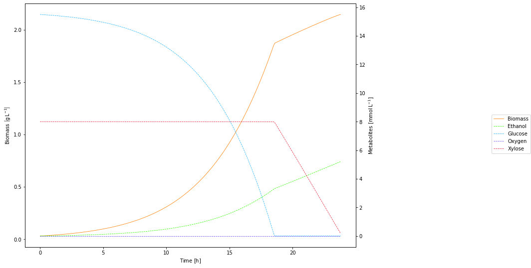
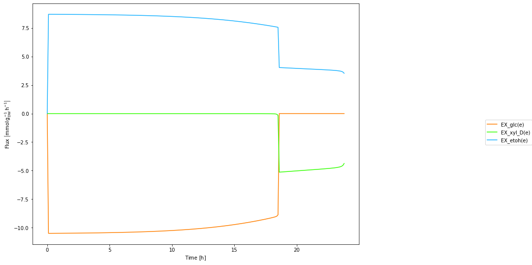
The model is simulated using the simulate method. This simulation covers the interval \([0.0, 25.0]\) hours, with results stored every \(0.1\) hours. Results (trajectories of kinetic variables) will be returned as pandas.DataFrame. Optionally, the user can also provide a list of reaction ids whose flux trajectories will also be returned as a separate pandas.DataFrame, in this case three exchange fluxes in the model.

dfba_model.add_initial_conditions(
    {
        "Biomass": 0.03,
        "Glucose": 15.5,
        "Xylose": 8.0,
        "Oxygen": 0.0,
        "Ethanol": 0.0,
    }
)
concentrations, trajectories = dfba_model.simulate(0.0, 25.0, 0.1, ["EX_glc(e)", "EX_xyl_D(e)", "EX_etoh(e)"])

7. Plotting the results

Note: In order to plot the results, one of plotly or matplotlib should be used. See Visualization to install them along with dfba.

Plotly

The functions for plotting with plotly returns a plotly.graph_object. Users of this library may plot the output with the usual functions.

from dfba.plot.plotly import *

import plotly.io as pio

# in plotly version 4, default version is different than in 3
pio.templates.default = "plotly_white"

fig = plot_concentrations(concentrations)
fig.show()

fig = plot_trajectories(trajectories)
fig.show()

Matplotlib

We can use the matplotlib backend with the same functions.

from dfba.plot.matplotlib import *

%matplotlib inline
import matplotlib.pyplot as plt
plt.rcParams["figure.figsize"] = 16, 9

plot_concentrations(concentrations)
plt.show()

plot_trajectories(trajectories)
plt.show()

8. Writing the results to file

Particularly when running a simulation using Docker (see Installation), it can be useful to write results to a csv file for downstream analysis. This can be achieved using the pandas.DataFrame method to_csv()

concentrations.to_csv("concentrations.csv")
trajectories.to_csv("trajectories.csv")